Model Descriptions

Model Descriptions#

CIOFS Models#

There are three models being actively run in and/or used in Cook Inlet which are all referred to as CIOFS models since they use the same grid and domain:

CIOFS operational: Run as a nowcast/forecast since Aug 31, 2021 and forecast 48 hours. Portal link
CIOFS hindcast: from 1999 through 2022. Portal link
CIOFS freshwater forcing: 2003–2006 and 2012–2014. Portal link

where CIOFS originally stood for Cook Inlet Operational Forecast System.

https://ciofs.axds.co/_images/ciofs_bathy.png — Fig. 1 Bathymetry for all CIOFS models.#

All CIOFS models are run using Regional Ocean Modeling System (ROMS) [Shchepetkin and McWilliams [SM05], McWilliams [McW09]] using the same horizontal grid and number of vertical levels and stretching/transform functions (see bathymetry in Fig. 1). The horizontal grid ranges from 10 meters to 3.5 kilometers resolution and the vertical grid has 30 sigma levels with Vstretching=1 and Vtransform=1.

Since the current project uses output from the CIOFS hindcast and freshwater models (see example animation in Fig. 2), we will present the forcing for those models here.

_images/ciofs_freshwater.mp4

Fig. 2 Example animation showing the surface salinity for CIOFS Hindcast (left) and CIOFS Freshwater (right).#

Both CIOFS Hindcast and CIOFS Freshwater#

Time-varying surface forcing for both models comes from ECMWF Reanalysis v5 (ERA5) for wind, temperature, and humidity [HBB+20]. Boundary forcing is from HYCOM Global Ocean Forecasting System (GOFS) 3.1 Reanalysis and is for temperature, salinity, and sub-tidal water levels [NavalRLaboratory21]. The open boundary forcing for tides is from the NOS CO-OPS version of CIOFS [NOAA [NOA19]; Zhang [Zha19]] which is derived from the ADCIRC tidal database [ADCd.].

Each modeling period required a 1 year spin up time period that was discarded.

The difference between the two models was in how the freshwater forcing was implemented. That is described in the following sections for each model.

CIOFS Hindcast#

The CIOFS Hindcast model used river inputs with real-time discharge observations from 12 major rivers supplied by the USGS for freshwater forcing [USGS16].

Additional details about the CIOFS Hindcast model forcing are included in the original CIOFS Hindcast report [TLFD23].

CIOFS Freshwater-Forced#

Hydrology Model#

The CIOFS Freshwater model used output from a watershed model as the freshwater forcing, similar to what is described in [DHH+20]. The hydrology model of the Gulf of Alaska watershed provided by David Hill, Oregon State University [[BHAL16], [HBC+15]] was used to create the ROMS river (point sources) input files. The data made available to Axiom contains daily discharge values at coastal grid points along the Gulf of Alaska from the hydrology model’s native grid.

Python scripts created by Kate Hedstrom were used to generate the ROMS point source input files for the CIOFS freshwater hindcast. The scripts transform the discharge values from the hydrology model into a ROMS grid-specific format, including identifying discharge points in the ROMS grid, mapping and re-indexing discharge values from the input points to ROMS discharge points, and other necessary calculations to prepare the data for the ROMS model. Modifications to the scripts were made so that the generated input files work with the CIOFS grid. An additional measure to increase the model stability was to redistribute extremely high discharge at a single point across several nearby points. To account for large discharge from point sources, the maximum speed in ROMS was increased from 20 to 80 m/s by modifying mod_scalars.F in ROMS source code, following the ROMS manual [Hedstrom18].

The resulting difference in the total amount of volumetric rate of freshwater input for each model is shown in Fig. 3.

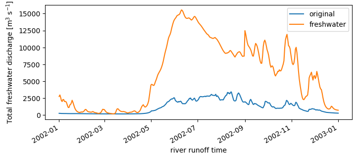
_images/freshwater_input.png — Fig. 3 Overall freshwater input for CIOFS Hindcast (blue) and CIOFS Freshwater (orange) models for the first year of spin-up time, 2002.#

Computation#

The CIOFS freshwater simulations were performed using the Intel Fortran Compiler and Intel MPI, which are provided in the oneAPI base toolkit and HPC toolkit, version 2023, for parallelization on a local cluster consisting of 23 nodes. A total of 9 nodes each contained 40 Intel Xeon Gold 6148 (Skylake) CPU cores, allowing for a total of 360 cores to perform the 2003-2006 simulation. The remaining 14 nodes each contained 48 Intel Xeon Gold 6262 (Cascade Lake) CPU cores, allowing for a total of 672 cores to perform the 2012-2014 simulation. Both model simulations were performed concurrently. Nodes were connected via QDR InfiniBand fabric, which enabled the two groups of hindcast simulations over 7 years in total to complete within one and a half months. This performance demonstrates efficient scaling, enabling the high-resolution simulations required for this project to be feasibly executed within a reasonable timeframe. The Intel compiler and MPI implementation tailored for the Xeon architecture was critical in maximizing utilization of the available compute capability.