Methodology#
Software#
The datasets are compared with model output from the CIOFS and NWGOA models using the ocean-model-skill-assessor (OMSA) framework, as well as dependencies therein and software written for this report. Detailed documentation is available for OMSA.
Taylor Diagram#
Taylor diagrams are used to summarize in one diagram several pieces of information about how accurately a model captures the behavior in a set of observations [Tay01]. They directly represent the correlation coefficient and the standard deviation of the model and observations, and due to geometric relationships, also the root mean squared error. Taylor diagrams are used to demonstrate the overall performance of the models in this study by concatenating all comparisons of a type (e.g., all CTD transects) and calculating the metrics to use in the diagram using the single concatenated model and data representations. The Taylor Diagram uses code from Copin [Cop12].
By Region#
We split Cook Inlet into regions to give some spatial information in the region-based Taylor diagrams. The resulting regions are shown in Fig. 24.
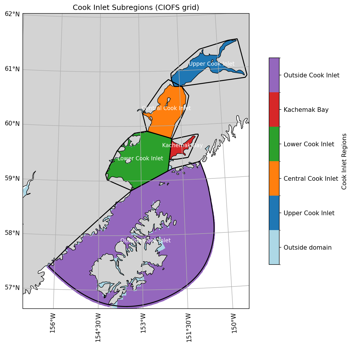
Fig. 24 Cook Inlet, split into named regions for analysis.#
By Season#
We split the year into seasons for grouping by time, defined as follows:
Winter: December through March
Spring: April and May
Summer: June through August
Fall: September through November
Comparison Metrics#
Multiple statistical measures of the model-data comparison are given, though skill score is used as the main overview measure. To compare model and data output, the model output was interpolated in time and space to match the data.
All Metrics#
The available statistical metrics are:
Bias
Correlation coefficient
Index of agreement
Root mean square error (RMSE)
Skill score (SS)
Bias#
The bias (the mean of the difference) is defined as:
\( \text{Bias} = \frac{1}{N} \sum_{i=1}^{N} \left( M_i - O_i \right), \)
where \(M_i\) is the model value at index \(i\), \(O_i\) is the corresponding observation, and \(N\) is the total number of paired samples. A positive bias indicates the model overestimating the observations and a negative bias represents the model underestimating the observations.
Correlation Coefficient#
The correlation coefficient [Pea95] is defined as:
\(r = \frac{\sum_{i=1}^N \left( M_i - \overline{M} \right) \left( O_i - \overline{O} \right)}{\sqrt{\sum_{i=1}^N \left( M_i - \overline{M} \right)^2} \ \sqrt{\sum_{i=1}^N \left( O_i - \overline{O} \right)^2}}\)
where \(M_i\) is the model value at index \(i\), \(O_i\) is the corresponding observation, \(\overline{M}\) is the mean of the model values, \(\overline{O}\) is the mean of the observations, and \(N\) is the total number of paired samples. The correlation coefficient measures how much the model follows the temporal patterns of the observations and ranges from -1 (exactly negative linear relationship) to 1 (exactly positive linear relationship). Note that a model can have a correlation coefficient of 1 but still have a large bias.
Index of Agreement#
The index of agreement Willmott [Wil81] is defined as:
\(d = 1 - \frac{\sum_{i=1}^N \left( M_i - O_i \right)^2}{\sum_{i=1}^N \left( \left| M_i - \overline{O} \right| + \left| O_i - \overline{O} \right| \right)^2}\)
where \(M_i\) is the model value at index \(i\), \(O_i\) is the corresponding observation, \(\overline{O}\) is the mean of the observations, and \(N\) is the total number of paired samples. The index of agreement measures both the pattern and magnitude of the model as compared with the observations, and ranges from 0 (no agreement) to 1 (perfect agreement). Because it measures both magnitude and patterns, it is a useful combined metrics, but it is harder to interpret than a single metric like correlation and it is sensitive to outliers.
Root Mean Squared Error (RMSE)#
The root mean squared error (RMSE) is defined as:
\( \text{RMSE} = \sqrt{ \frac{1}{N} \sum_{i=1}^N (M_i - O_i)^2 }, \)
where \(M_i\) is the model value at index \(i\), \(O_i\) is the observation, and \(N\) is the total number of paired samples. The RMSE represents the model error relative to the observations, and is sensitive to outliers.
Skill score#
Taylor suggests a skill score \(SS\) in Taylor [Tay01] that combines the information in the Taylor diagram to represent model skill with a single value:
\( S = \frac{4 (1 + r)^4}{\left( \frac{\sigma_m}{\sigma_o} + \frac{1}{\sigma_m / \sigma_o} \right)^2 (1 + r_0)^4} \)
where \( \sigma_m \) is the standard deviation of the model, \( \sigma_o \) is the standard deviation of the observations, \( r \) is the correlation coefficient between the model and observations, and \( r_0 \) is the maximum attainable correlation coefficient (often taken as 1). The maximum attainable correlation coefficient accounts for the fact that variability inherent in the system means that no two models will ever be exactly the same without the exact same forcing. The skill score is 1 when the model variance is the same as the observational variance and there is perfect correlation, and can be down to -1 for negative correlation values.
Details of comparisons#
Units#
Variable |
Unit |
|---|---|
Sea water temperature |
Deg Celsius |
Sea water salinity |
PSU |
Sea surface height |
m |
Along/across-channel velocity |
m/s |
Speed |
m/s |
Comparisons shown#
One or more of the following time series modifications is used where noted to alter the data and model time series before comparison. Detailed explanations of each are given below, and which have been used are noted for each model-data comparison.
Tidal filtering#
The tides are an important feature of Cook Inlet, and if we do not remove them from the time series we want to compare, they will dominate the model-data comparisons. Because the tides have a highly correlated signal, comparing time series with them intact from moment to moment gives a skewed comparison; if the model-data comparison at one time is close, it probably will also be at the next time. A better way to compare the model and data in a regime like this is by first filtering out the tides; we use the pl33 filter to do so. We filter out the tides for most model-data comparisons presented here, though if a sea surface height time series is relatively short, we left it with tides to show the full comparison.
Long time series#
Long time series of temperature or salinity tend to have significant annual cycles. In a similar way to the tides, this can skew the meaning of our statistical metrics because, for example, the large, expected temperature cycle dominates any smaller features. Because of this, we present long time series of temperature and salinity as the anomaly with respect to the monthly mean calculated from the data time series across the available years. We will often also show the comparisons without removing the monthly mean to help give an intuitive feel for how the model is behaving with respect to the data.
Mean subtracted#
Numerical ocean models tend to not have a specific vertical datum that they are calculated with respect to. For this reason, when the sea surface height is compared between model and data, the mean of each is separately subtracted from the time series before comparison.
Harmonic tidal analysis#
Harmonic tidal analysis was run to calculated tidal constants with the HF Radar data. We ran a Python version of the classic Matlab package T_Tide [PBL02].
How to read a model-data figure#
Consider the example model-data comparison in Fig. 25 for a year of mooring data. The title contains a lot of information:
station identifier
statistical metric values
bias
correlation coefficient (“corr”)
index of agreement (“ioa”)
root mean squared error (“rmse”)
skill score (“ss”)
distance of model grid-node from actual data location, if relevant (“dist”)
standard deviation of the model and observations (std\(_M\), std\(_O\))
date or start date of observations
depth or first depth
longitude and latitude location (“lon” and “lat”)
descriptive title
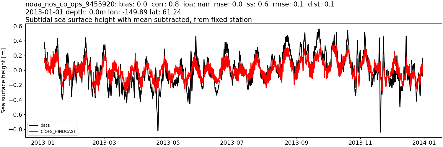
Fig. 25 Example of CIOFS Freshwater subtidal time series comparison with sea surface height data (Station noaa_nos_co_ops_9455920).#